
LINEAR FUNCTIONS
By: Carly Cantrell
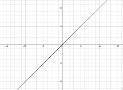
Let’s explore the two linear functions given below:
f(x) = x + 1
g(x) = x – 1
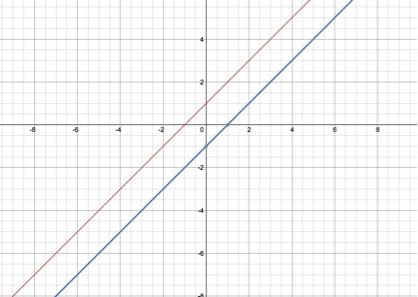
The above graph shows two linear functions. These functions are parallel because they have the same slope. The slope of f(x) and g(x) are both 1. These functions differ by a single translation. Compared to the parent function, f(x) is translated up one unit and g(x) is translated down one unit. The next graph shows the summative relationship of f(x) and g(x).
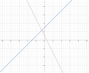
The sum of the two functions:
h(x) = f(x) + g(x)
h(x) = x + 1 + x – 1
h(x) = 2x
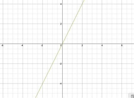
This function remains linear because two linear functions were added together, which results in a single linear function. This new function, h(x), has a slope greater than either of the original functions. The slope increases at a rate twice as fast because the original two functions both had the slope of 1. Now, this function has a slope of 2. Notice, h(x) goes through the origin. Neither, f(x) or g(x) went through the origin. The reason h(x) goes through the origin is because the original functions were equidistant away from the origin in opposite directions. The next graph will show the multiplicative relationship between f(x) and g(x).
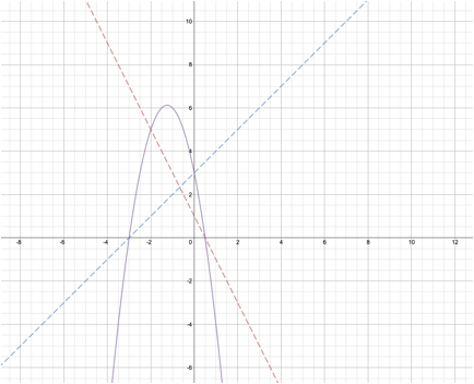
The product of the two functions:
h(x) = f(x)*g(x)
h(x) = (x+1)(x-1)
h(x) = x2 -1
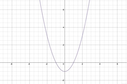
This function is no longer linear! In fact, this is now a quadratic function. The graph shown above is a parabola. This particular function has a minimum because the parabola opens upwards. The domain of quadratic functions will always be all real numbers, while the range depends on the specific function. This function has two roots, one at x = -1 and the second at x = 1. The minimum is located at the vertex: (0,-1). This is shown in the function h(x) = x2 – 1. The shift downwards justifies the location of the vertex and the reason for having two roots. Next, we will look at the quotient of the two original linear functions.
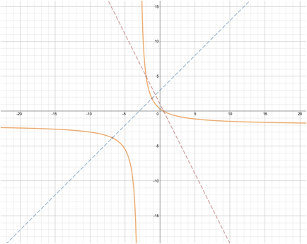
h(x) = ![]()
h(x) =![]()
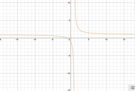
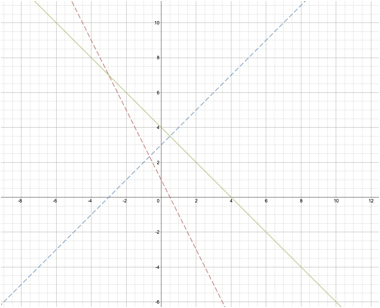
This function becomes a rational function. First, the domain
of a rational function consists of all real numbers except the zeroes of the
polynomial in the denominator. The
graph takes on the shape from above because this function contains both a
vertical and horizontal asymptote. Vertical asymptotes are the imaginary
vertical lines that form boundaries in the graph. The is where the function is
undefined; the vertical asymptote for h(x) is x=1. This is
shown in the graph above because the function gets very close to x=1, while
never touching it. Horizontal asymptotes are very similar. Horizontal
asymptotes are imaginary horizontal lines that the graph will approach as x
increase or decreases to ![]() .
The horizontal asymptotes for the function h(x) is
y=1 because the degree of the leading coefficients are equal and both 1. When
the degrees are equal you divide the coefficients, respectively, hence for h(x) it is 1 / 1 = 1.
.
The horizontal asymptotes for the function h(x) is
y=1 because the degree of the leading coefficients are equal and both 1. When
the degrees are equal you divide the coefficients, respectively, hence for h(x) it is 1 / 1 = 1.
The composition of the two functions:
h(x) = f(g(x))
h(x) = (x – 1) + 1
h(x) = x
This function remains a linear function because each of these original functions was linear. Will this always be the case?
Let’s look at the same relationships using different linear functions:
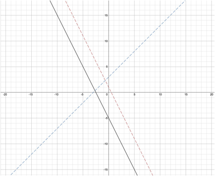
Let’s try two linear functions with different and opposite slopes:
f(x)= -2x+1
g(x)= x+3
Summative Relationship:
h(x)= f(x)+g(x)
Multiplicative Relationship:
h(x)= f(x)*g(x)
Quotient Relationship:
h(x)=![]()
Composed Relationship:
h(x)= f(g(x))
In summary, the same relationship upheld when the two linear function were changed. When adding two linear functions, the result is a different linear function. When multiplying two linear functions, the result is a quadratic function. When dividing two linear functions, the result is a rational function. Lastly, when composing two linear functions, the result is a different linear function.